Implement a new power flow surrogate
This tutorial shows how to implement a new power flow surrogate based on [Bernstein2017].
The purpose of a power flow surrogate is to relate direct variables (voltage at PCC and power injections at PQ buses) to indirect variables (power injection at PCC and voltage at PQ buses). Concretely, the power flow surrogate needs to implement the following constraints:
- Voltage magnitude limits
- Power injection at PCC
In addition, the surrogate needs to specify the voltage at PCC. At first, this might seem surprising since the voltage at PCC is a direct variable. However, recall that different surrogates represent voltage in different ways. For example:
uot.PowerFlowSurrogate_Gan2014_SDPuses one hermitian matrix per busuot.PowerFlowSurrogate_Bolognani2015_LPuses one real vector for voltage magnitude and another for voltage phase
This means, the implementation of the voltage at PCC constraint is different in each case. Consequently, UOT leaves the implementation of the constraint to each surrogate.
The opposite happens for the power injection at the PCC: it is an indirect variable but the constraints on it are implemented by uot.ControllableLoad and not by the surrogate.
The reason is that the PCC load is always represented in the same way: one real vector for active power injection and another for reactive power injection.
Since the constraints always take the same form, it makes sense to implement them only once.
One important remark is in order: the PCC load is implemented in uot.OPFproblem but the power flow surrogate must couple it to the rest of the problem through a constraint. This is typically done through:
[P_inj_array,Q_inj_array] = obj.opf_problem.ComputeNodalPowerInjection();
For an example, see uot.PowerflowSurrogate_Bolognani2015_LP.GetConstraintArray.
Power flow surrogate specification
The first step is creating PowerFlowSurrogateSpec_Bernstein2017_LP_1 which is a derived class of uot.AbstractPowerFlowSurrogateSpec.
A good starting point is making a copy of uot.SpecTemplate and changing the parent class to uot.AbstractPowerFlowSurrogateSpec.
By convention, we put the class in a directory named @PowerFlowSurrogateSpec_Bernstein2017_LP_1.
This is not strictly necessary but makes it easier to see if a file is a class, function or script.
For now, we can leave the sample documentation as it is.
Looking at uot.AbstractPowerFlowSurrogateSpec, we learn that the purpose of PowerFlowSurrogateSpec_Bernstein2017_LP_1 is simply telling uot.OPFproblem how to instantiate the power flow surrogate.
For this purpose, we need to create a concrete implementation of uot.AbstractPowerFlowSurrogateSpec.Create.
For inspiration, we can look how this is done in uot.PowerFlowSurrogateSpec_Bolognani2015_LP.
At the end, we have:
1 2 3 4 5 6 7 8 9 10 11 12 13 14 15 16 17 18 19 20 21 22 23 24 25 26 27 28 29 30 31 32 33 34 35 36 37 38 39 40 41 42 43 44 45 46 47 48 49 50 51 52 53 54 55 | classdef PowerFlowSurrogateSpec_Bernstein2017_LP_1 < uot.AbstractPowerFlowSurrogateSpec
% Class to specify xx
%
% Synopsis::
%
% obj = uot.SpecTemplate(bus,varargin)
%
% Description:
% This class is intended as a starting point to develop classes that
% derive from ``uot.Spec``.
%
%
% We can also itemize
%
% - item 1
% - item 2
%
%
% Arguments:
% bus (char): Bus name
%
% Keyword Arguments:
% 'param1': Something.
%
% Returns:
% obj: Instance of `uot.SpecTemplate`.
%
% Note:
% Possibly add a note here
%
% Example::
%
% object = uot.ObjectTemplate(uot.SpecTemplate())
%
% See Also:
% `uot.ObjectTemplate`
%
% Todo:
%
% - Write documentation
%
% .. Line with 80 characters for reference #####################################
methods
function obj = PowerFlowSurrogateSpec_Bernstein2017_LP_1()
end
end
% Implemented abstract methods from uot.AbstractPowerFlowSurrogateSpec
methods
function pf_surrogate = Create(obj,varargin)
pf_surrogate = PowerFlowSurrogate_Bernstein2017_LP_1(obj,varargin{:});
end
end
end
|
Note
We add the suffix _1 to distinguish this first implementation from more evolved ones we will develop in the course of the tutorial.
Note
The classes created in this tutorial are not prefixed by uot, since they are not in the +uot directory which builds the module. The production implementation (which is preceded by uot) are optimized for performance and include further functionality which is outside the scope of this tutorial
Barebones power flow surrogate
The next step is creating a barebones power flow surrogate class which is derived of uot.AbstractPowerFlowSurrogate.
Looking at uot.AbstractPowerFlowSurrogate, we see that we need to implement some abstract methods:
AssignBaseCaseSolution()ComputeVoltageEstimate()GetConstraintArray()SolveApproxPowerFlow()(static)
We now create the class PowerFlowSurrogateSpec_Bernstein2017_LP_1 with these methods as stubs.
A good starting point is making a copy of uot.ObjectTemplate and changing the parent class to uot.AbstractPowerFlowSurrogate.
For now, we can leave the sample documentation as it is.
We implement the constructor following the example of uot.PowerFlowSurrogate_Bolognani2015_LP.
At the end, we have the barebones implementation:
1 2 3 4 5 6 7 8 9 10 11 12 13 14 15 16 17 18 19 20 21 22 23 24 25 26 27 28 29 30 31 32 33 34 35 36 37 38 39 40 41 42 43 44 45 46 47 48 49 50 51 52 53 54 55 56 57 58 59 60 61 | classdef PowerFlowSurrogate_Bernstein2017_LP_1 < uot.AbstractPowerFlowSurrogate
% Template class for uot.Object.
%
% Synopsis::
%
% obj = uot.ObjectTemplate(spec,'param1',val1)
%
% Description:
% This class is intended as a starting point to develop classes that
% derive from ``uot.Object``.
%
%
% We can also itemize
%
% - item 1
% - item 2
%
% Arguments:
% spec (|uot.SpecTemplate|): Object specification
%
% Keyword Arguments:
% 'param1' (:class:`uot.PCCloadSpec<+uot.@PCCloadSpec.PCCloadSpec>`): Parameter
%
%
% Note:
% Possibly add a note here
%
% Example::
%
% object = uot.ObjectTemplate(uot.SpecTemplate())
%
% See Also:
% |uot.SpecTemplate|
%
% Todo:
%
% - Write documentation
%
% .. Line with 80 characters for reference #####################################
methods
function obj = PowerFlowSurrogate_Bernstein2017_LP_1(spec,opf_problem)
validateattributes(spec,{'PowerFlowSurrogateSpec_Bernstein2017_LP_1'},{'scalar'},mfilename,'spec',1);
decision_variables = [];
obj@uot.AbstractPowerFlowSurrogate(spec,opf_problem,decision_variables)
end
constraint_array = GetConstraintArray(obj) % Abstract method from uot.AbstractPowerFlowSurrogate
end
methods (Static)
[U_array,T_array,p_pcc_array,q_pcc_array,opf_problem] = SolveApproxPowerFlow(load_case,u_pcc_array,t_pcc_array) % Abstract method from uot.AbstractPowerFlowSurrogate class
end
methods (Access = {?uot.AbstractPowerFlowSurrogate,?uot.OPFproblem})
[U_array,T_array,p_pcc_array,q_pcc_array] = AssignBaseCaseSolution(obj) % Abstract method from uot.AbstractPowerFlowSurrogate
[U_array,T_array] = ComputeVoltageEstimate(obj) % Abstract method from uot.AbstractPowerFlowSurrogate
end
end
|
Initialize OPF problem with PowerFlowSurrogateSpec_Bernstein2017_LP_1
Here, we instantiate OPF problem with PowerFlowSurrogateSpec_Bernstein2017_LP_1 to verify that out barebones implementation is working as expected.
Generated from aaInstantiateBarebones.m
clear variables

aaSetupPath

[opf_spec, load_case] = CreateSampleOPFspec();

% Replace pf_surrogate_spec with PowerFlowSurrogateSpec_Bernstein2017_LP_1
opf_spec.pf_surrogate_spec = PowerFlowSurrogateSpec_Bernstein2017_LP_1();

opf_problem = uot.OPFproblem(opf_spec,load_case);
Note
By convention, we use the prefix aa in scripts to distinguish them from functions
Solving approximate power flow
Implementing power flow surrogates is tricky and error-prone. Hence, testing is an integral part of the process. One sensible way of doing this is trying to replicate the results in the paper.
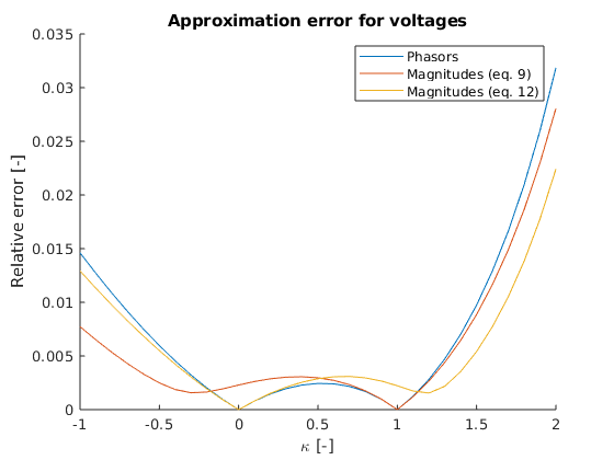
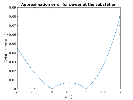
The paper presents a continuation analysis where they approximately solve power flow for a series of scaled loads using the proposed linear formulation. Then, they compare the results with the actual power flow solution and compute the error.
We will try to replicate the results in Figures 3 and 5 of the paper. Figure 3 shows an error of less than 0.2% in voltage whereas Figure 5 shows an error of less than 1.5% for the power at the PCC.
In order to replicate the paper’s results, we need to solve power flow and not optimal power flow.
It is very common that power flow surrogates offer a way of approximately solving power flow algebraically.
In fact, Bernstein’s paper is not about OPF at all.
The method uot.AbstractPowerFlowSurrogate.SolveApproxPowerFlowAlt exists precisely for this use case.
It can be overridden by a power flow surrogate to offer a way of solving power flow.
Note
The Alt in SolveApproxPowerFlowAlt is there because uot.AbstractPowerFlowSurrogate.SolveApproxPowerFlow also exists.
However, SolveApproxPowerFlow uses a different method that requires solving an optimization problem.
The advantage of the optimization-based method is that it works even for surrogates where power flow cannot be solved in an algebraic fashion (e.g., uot.PowerFlowSurrogate_Gan2014_SDP)
For this purpose, we implement PowerFlowSurrogate_Bernstein2017_LP_2.SolveApproxPowerFlowAlt():
1 2 3 4 5 6 7 8 9 10 11 12 13 14 15 16 17 18 19 20 21 22 23 24 25 26 27 28 29 30 31 32 33 34 35 36 37 38 39 40 41 42 43 44 45 46 47 48 49 50 51 52 53 54 55 56 57 58 59 60 61 62 63 64 65 66 67 68 69 70 71 72 73 74 75 76 77 78 79 80 81 82 83 84 85 86 87 88 89 90 91 92 93 94 95 96 97 98 99 100 101 102 103 104 105 106 107 108 109 110 111 112 113 114 115 116 117 118 119 120 121 122 123 124 125 126 | function [U_array,T_array, p_pcc_array, q_pcc_array,extra_data] = SolveApproxPowerFlowAlt(load_case,u_pcc_array,t_pcc_array,varargin)
% This function is static
% [...] = SolveApproxPowerFlowAlt(load_case,u_pcc_array,t_pcc_array) linearization at the flat voltage solution
% [...] = SolveApproxPowerFlowAlt(load_case,u_pcc_array,t_pcc_array,U_ast,T_ast) linearization at U_ast,T_ast
% Check inputs following how it's done in uot.PowerFlowSurrogate_Bolognani2015_LP.SolveApproxPowerFlowAlt
validateattributes(load_case,{'uot.LoadCasePy'},{'scalar'},mfilename,'load_case',1);
network = load_case.network;
n_time_step = load_case.spec.n_time_step;
n_phase = network.n_phase;
validateattributes(u_pcc_array,{'double'},{'size',[n_time_step,n_phase]},mfilename,'u_pcc_array',2);
validateattributes(t_pcc_array,{'double'},{'size',[n_time_step,n_phase]},mfilename,'t_pcc_array',3);
n_varargin = numel(varargin);
switch n_varargin
case 0
% Linearize at flat voltage
linearization_point = uot.enum.CommonLinearizationPoints.FlatVoltage;
[U_ast,T_ast] = linearization_point.GetVoltageAtLinearizationPoint(load_case,u_pcc_array,t_pcc_array);
case 2
U_ast = varargin{1};
T_ast = varargin{2};
validate_phase_consistency_h = @(x) uot.AssertPhaseConsistency(x,network.bus_has_phase);
uot.ValidateAttributes(U_ast,{'double'},{'size',[nan,nan,1],validate_phase_consistency_h},mfilename,'U_ast',4);
uot.ValidateAttributes(T_ast,{'double'},{'size',[nan,nan,1],validate_phase_consistency_h},mfilename,'T_ast',5);
otherwise
error('Invalid number of arguments.')
end
% Compute x_y
% Loads are negative power injections
S_inj_array = -load_case.S_y;
P_inj_array = real(S_inj_array);
Q_inj_array = imag(S_inj_array);
% x_y is the phase-consistent stack (see glossary) excluding the pcc (bus 1)
x_y = [uot.StackPhaseConsistent(P_inj_array(2:end,:,:),network.bus_has_phase(2:end,:,:));uot.StackPhaseConsistent(Q_inj_array(2:end,:,:),network.bus_has_phase(2:end,:,:))];
V_ast = uot.PolarToComplex(U_ast,T_ast);
% Remove pcc
V_ast_nopcc_stack = uot.StackPhaseConsistent(V_ast(2:end,:,:),network.bus_has_phase(2:end,:,:));
[P_ast,Q_ast] = network.ComputePowerInjectionFromVoltage(U_ast,T_ast);
x_y_ast = [uot.StackPhaseConsistent(P_ast(2:end,:,:),network.bus_has_phase(2:end,:,:));uot.StackPhaseConsistent(Q_ast(2:end,:,:),network.bus_has_phase(2:end,:,:))];
[~,~,w] = network.ComputeNoLoadVoltage(u_pcc_array,t_pcc_array);
% Compute voltage according to eq. 5a
Ybus_NN_inv = inv(network.Ybus_NN);
M_y_pre = Ybus_NN_inv*inv(diag(conj(V_ast_nopcc_stack)));
M_y = [M_y_pre,-1i*M_y_pre];
a = w;
V_nopcc_array_stack = M_y*x_y + a;
% Add pcc voltage
v_pcc_array = uot.PolarToComplex(u_pcc_array,t_pcc_array);
V_array_stack = [v_pcc_array.';V_nopcc_array_stack];
V_array = uot.UnstackPhaseConsistent(V_array_stack,network.bus_has_phase);
[U_array,T_array] = uot.ComplexToPolar(V_array);
% Compute pcc power injection according to eq. 5c and 13
s_pcc_array = zeros(n_time_step,network.n_phase);
for i = 1:n_time_step
v_pcc_i = v_pcc_array(i,:).';
G_y = diag(v_pcc_i)*conj(network.Ybus_SN)*conj(M_y);
c = diag(v_pcc_i)*(conj(network.Ybus_SS)*conj(v_pcc_i) + conj(network.Ybus_SN)*conj(a(:,i)));
s_pcc_array(i,:) = G_y*x_y(:,i) + c;
end
p_pcc_array = real(s_pcc_array);
q_pcc_array = imag(s_pcc_array);
% In addition to the results from standard power flow, the paper
% presents 2 approaches to approximate the magnitude of the voltages in the
% PQ nodes: using eq. 9 and eq. 12.
% We include them here so that we can test them.
% Approach from eq. 9
V_ast_nopcc_stack_abs = abs(V_ast_nopcc_stack);
K_y_eq9 = inv(diag(V_ast_nopcc_stack_abs))*real(diag(conj(V_ast_nopcc_stack))*M_y);
b_eq9 = V_ast_nopcc_stack_abs - K_y_eq9*x_y_ast;
U_array_stack_pre_eq9 = K_y_eq9*x_y + b_eq9;
U_array_stack_eq9 = [u_pcc_array.';U_array_stack_pre_eq9];
U_array_eq9 = uot.UnstackPhaseConsistent(U_array_stack_eq9,network.bus_has_phase);
% Approach from eq. 12
U_array_eq12 = zeros(network.n_bus,network.n_phase,n_time_step);
for i = 1:n_time_step
w_i = w(:,i);
W = diag(w_i);
K_y_eq12 = abs(W)*real(inv(W)*M_y);
b_eq12 = abs(w_i);
U_stack_pre_eq12 = K_y_eq12*x_y(:,i) + b_eq12;
U_stack_eq12 = [u_pcc_array(i,:).';U_stack_pre_eq12];
U_array_eq12(:,:,i) = uot.UnstackPhaseConsistent(U_stack_eq12,network.bus_has_phase);
end
extra_data.U_array_eq9 = U_array_eq9;
extra_data.U_array_eq12 = U_array_eq12;
end
|
Replicate the paper’s results to verify correctness
This file replicates the results in Figures 3 and 5 of [Bernstein2017].
Generated from aaReplicatePaperResults.m
clear variables
aaSetupPath
Initialize OPF problem with PowerFlowSurrogate_Bernstein2017_LP
[opf_spec, load_case] = CreateSampleOPFspec();

% Replace pf_surrogate_spec with PowerFlowSurrogateSpec_Bernstein2017_LP_2
opf_spec.pf_surrogate_spec = PowerFlowSurrogateSpec_Bernstein2017_LP_2();

opf_problem = uot.OPFproblem(opf_spec,load_case);
Solve approximate power flow to see if everything is working
linearization_point = uot.enum.CommonLinearizationPoints.FlatVoltage;

u_pcc_array = opf_problem.u_pcc_array;
t_pcc_array = opf_problem.t_pcc_array;

[U_ast,T_ast] = linearization_point.GetVoltageAtLinearizationPoint(load_case,u_pcc_array,t_pcc_array);
[U_array,T_array, p_pcc_array, q_pcc_array,extra_data] = PowerFlowSurrogate_Bernstein2017_LP_2.SolveApproxPowerFlowAlt(load_case,u_pcc_array,t_pcc_array,U_ast,T_ast);
Set-up for continuation analysis
Now, we will try to replicate the paper’s results. In the continuation analysis, the authors used a range of factors kappa in [-1,2]
kappa_vec = -1:0.1:2;

% We reorder kappa_vec so that 1 is the first element.
% The reason for this is explained below.
kappa_vec = [kappa_vec(kappa_vec == 1), kappa_vec(kappa_vec ~= 1)];

% Then we use kappa_vec to create a load_case which is scaled
% according to kappa_vec. This works because load_case contains loads for
% a single time-step (as in the IEEE specification).
load_case_continuation = load_case.*kappa_vec;

% The result is a load case with loads for n_time_step
% time steps. Here, they do not represent actual time steps, but rather
% the different loads for our continuation analysis. We take advantage
% of the capability of representing time-varying loads to make the code
% more concise.
n_time_step = load_case_continuation.n_time_step
n_time_step =

    31
Choose a linearization point
Now we need to choose a linearization point for solving the approximate power flow. One common choice is the power flow solution at the first time of the base case. Here, the base case should be understood in the context of OPF problems: the case in the absence of controllable loads. However, since we are not working with controllable loads yet, this is simply the first time step of the load case. Here, it should become clear why we reordered kappa_vec above so that 1 is the first element: so that we use it as our linearization point.
linearization_point_continuation = uot.enum.CommonLinearizationPoints.PFbaseCaseFirstTimeStep;
Solve approximate power flow using the linear formulation
Extend u_pcc_array and t_pcc_array to have one entry per time step
u_pcc_array_continuation = repmat(u_pcc_array,n_time_step,1);
t_pcc_array_continuation = repmat(t_pcc_array,n_time_step,1);

[U_ast_continuation,T_ast_continuation] = linearization_point_continuation.GetVoltageAtLinearizationPoint(load_case_continuation,u_pcc_array_continuation,t_pcc_array_continuation);
[U_array_continuation,T_array_continuation, p_pcc_array_continuation, q_pcc_array_continuation,extra_data_continuation] = PowerFlowSurrogate_Bernstein2017_LP_2.SolveApproxPowerFlowAlt(load_case_continuation,u_pcc_array_continuation,t_pcc_array_continuation,U_ast_continuation,T_ast_continuation);

V_array_continuation = uot.PolarToComplex(U_array_continuation,T_array_continuation);
s_pcc_continuation = p_pcc_array_continuation + 1i*q_pcc_array_continuation;
Get reference values from solving exact power flow
[U_array_ref,T_array_ref, p_pcc_array_ref, q_pcc_array_ref] = load_case_continuation.SolvePowerFlow(u_pcc_array_continuation,t_pcc_array_continuation);

V_array_ref = uot.PolarToComplex(U_array_ref,T_array_ref);
s_pcc_ref = p_pcc_array_ref + 1i*q_pcc_array_ref;
Compute error
v_error = zeros(n_time_step,1);
u_error_eq9 = zeros(n_time_step,1);
u_error_eq12 = zeros(n_time_step,1);
s_pcc_error_pre = zeros(n_time_step,1);

network = load_case_continuation.network;

for i = 1:n_time_step
    % Stack to get a vector without nans
    V_continuation_stack = uot.StackPhaseConsistent(V_array_continuation(:,:,i),network.bus_has_phase);
    V_ref_stack = uot.StackPhaseConsistent(V_array_ref(:,:,i),network.bus_has_phase);

    U_continuation_eq9_stack = uot.StackPhaseConsistent(extra_data_continuation.U_array_eq9(:,:,i),network.bus_has_phase);
    U_continuation_eq12_stack = uot.StackPhaseConsistent(extra_data_continuation.U_array_eq12(:,:,i),network.bus_has_phase);

    U_ref_stack = uot.StackPhaseConsistent(U_array_ref(:,:,i),network.bus_has_phase);

    v_error(i) = norm(V_continuation_stack - V_ref_stack,2)/norm(V_ref_stack,2);
    u_error_eq9(i) = norm(U_continuation_eq9_stack - U_ref_stack,2)/norm(U_ref_stack,2);
    u_error_eq12(i) = norm(U_continuation_eq12_stack - U_ref_stack,2)/norm(U_ref_stack,2);

    s_pcc_error_pre(i) = norm(s_pcc_continuation(i,:) - s_pcc_ref(i,:));
end

% Compute apparent power by summing across phases and taking absolute value.
s_pcc_mag_ref = abs(sum(s_pcc_ref,2));

s_pcc_error = s_pcc_error_pre/max(s_pcc_mag_ref);
Create plots
Sort kappa_vec to get a nice plot
[kappa_vec_sorted,kappa_vec_sorted_ind] = sort(kappa_vec);

v_error_sorted = v_error(kappa_vec_sorted_ind);
u_error_eq9_sorted = u_error_eq9(kappa_vec_sorted_ind);
u_error_eq12_sorted = u_error_eq12(kappa_vec_sorted_ind);

s_pcc_error_sorted = s_pcc_error(kappa_vec_sorted_ind);

% Compute error in voltage approximation
figure
hold on
plot(kappa_vec_sorted,v_error_sorted);
plot(kappa_vec_sorted,u_error_eq9_sorted);
plot(kappa_vec_sorted,u_error_eq12_sorted);
legend('Phasors','Magnitudes (eq. 9)','Magnitudes (eq. 12)')
title('Approximation error for voltages')
xlabel('\kappa [-]')
ylabel('Relative error [-]')

% Compute error in PCC power
figure
plot(kappa_vec_sorted,s_pcc_error_sorted);
title('Approximation error for power at the substation')
xlabel('\kappa [-]')
ylabel('Relative error [-]')
Creating an initial test case
We managed to replicate the results of the paper giving us trust in the correctness of our implementation.
The next step is to make a functional test case out of this experiment.
The starting point for this is SampleTest().
As before, we can take inspiration from other power flow surrogates, for example, PowerFlowSurrogate_Bolognani2015_LPtest() for inspiration.
This file has two test cases (i.e., functions starting with Test): TestAgainstPaper() and TestPowerFlowSurrogate_Bolognani2015_LP().
TestAgainstPaper() compares the results of the UOT implementation with code published by the paper’s authors.
This test is rooted on uot.PowerFlowSurrogate_Bolognani2015_LP.SolveApproxPowerFlowAlt.
PowerFlowSurrogate_Bolognani2015_LP() then verifies that the result of solving an OPF problem are consistent with uot.PowerFlowSurrogate_Bolognani2015_LP.SolveApproxPowerFlowAlt.
Furthermore, it verifies that constraints of the OPF problem are satisfied.
Now, we create a test case analogous to TestAgainstPaper based on our previous results:
1 2 3 4 5 6 7 8 9 10 11 12 13 14 15 16 17 18 19 20 21 22 23 24 25 26 27 28 29 30 31 32 33 34 35 36 37 38 39 40 41 42 43 44 45 46 47 48 49 50 51 52 53 54 55 56 57 58 59 60 61 62 63 64 65 66 67 68 69 70 71 72 73 74 75 76 77 78 79 80 | function tests = PowerFlowSurrogate_Bernstein2017_LP_2test
% Verifies that PowerFlowSurrogate_Bernstein2017_LP_2:
% - PowerFlowSurrogate_Bernstein2017_LP.SolveApproximatePowerFlowAlt can
% replicate the results in the original paper.
% This enables us to run the test directly instead of only through runtests
call_stack = dbstack;
% Call stack has only one element if function was called directly
if ~any(contains({call_stack.name},'runtests'))
this_file_name = mfilename();
runtests(this_file_name)
end
tests = functiontests(localfunctions);
end
function setupOnce(test_case)
aaSetupPath
test_case.TestData.abs_tol_equality = 5e-6;
end
function TestAgainstPaper(test_case)
load_case_zip = GetLoadCaseIEEE_13_NoRegs_Manual();
% Reference voltage from spec (we do not model the regulator)
u_pcc = [1.0625, 1.0500, 1.0687];
t_pcc = deg2rad([0, -120, 120]);
% Convert all loads to constant power wye-connected
load_case_pre = load_case_zip.ConvertToLoadCasePy();
% The paper uses kappa \in [-1,2]. However, we focus here on a narrower
% range where the approximate power flow is closest to the exact one.
kappa_vec = -0.2:0.1:1.2;
% Reorder kappa_vec so that kappa_vec(1) is 1.
% This, will allow us to linearize at the unscaled load
kappa_vec = [kappa_vec(kappa_vec == 1), kappa_vec(kappa_vec ~= 1)];
load_case = load_case_pre.*kappa_vec;
% Extend u_pcc_array and t_pcc_array to have one entry per time step
n_time_step = load_case.n_time_step;
u_pcc_array = repmat(u_pcc,n_time_step,1);
t_pcc_array = repmat(t_pcc,n_time_step,1);
linearization_point = uot.enum.CommonLinearizationPoints.PFbaseCaseFirstTimeStep;
[U_ast,T_ast] = linearization_point.GetVoltageAtLinearizationPoint(load_case,u_pcc_array,t_pcc_array);
[U_array,T_array, p_pcc_array, q_pcc_array,extra_data] = PowerFlowSurrogate_Bernstein2017_LP_3.SolveApproxPowerFlowAlt(load_case,u_pcc_array,t_pcc_array,U_ast,T_ast);
V_array = uot.PolarToComplex(U_array,T_array);
s_pcc = p_pcc_array + 1i*q_pcc_array;
% Get reference values from solving exact power flow
[U_array_ref,T_array_ref, p_pcc_array_ref, q_pcc_array_ref] = load_case.SolvePowerFlow(u_pcc_array,t_pcc_array);
V_array_ref = uot.PolarToComplex(U_array_ref,T_array_ref);
s_pcc_ref = p_pcc_array_ref + 1i*q_pcc_array_ref;
% We select the initial tolerance based on aaReplicatePaperResults and
% we tune them so that the tests just pass.
v_tol = 6e-3;
% For simplicity, we compare elementwise instead of using the paper's relative
% error metric. This will also issue a more informative error if the test fails.
% We use absolute tolerances because voltage magnitude is close to 1
verifyEqual(test_case,V_array,V_array_ref,'AbsTol',v_tol)
verifyEqual(test_case,extra_data.U_array_eq9,U_array_ref,'AbsTol',v_tol)
verifyEqual(test_case,extra_data.U_array_eq12,U_array_ref,'AbsTol',v_tol)
% We compare s_pcc using relative error because it is not necessarily close to 1
% Note that the tolerance is much larger than the 0.02 error we saw in the plot
% of aaReplicatePaperResults. This is because here we normalize with the actual
% load and not the maximal one as done in the paper. Thus the errors for the
% small loads (small kappa) are much larger than before.
s_pcc_tol = 0.15;
verifyEqual(test_case,s_pcc,s_pcc_ref,'RelTol',s_pcc_tol)
end
|
Implementing the power flow surrogate
Finally, we get to the implementation of the actual surrogate. For this purpose, we need to implement the following methods:
GetConstraintArrayHelper()DefineDecisionVariables()
Let’s get started with GetConstraintArrayHelper(), which defines the constraints we need to implement.
From above, we know these are:
- Voltage at PCC
- Voltage magnitude limits
- Power injection at PCC
Again, we can use uot.PowerFlowSurrogate_Bolognani2015_LP.GetConstraintArrayHelper for guidance.
Furthermore, we can use much of the code that we wrote for PowerFlowSurrogate_Bernstein2017_LP_2.SolveApproxPowerFlowAlt().
In order to reduce code duplication we will be moving some of the code there into new methods.
We just need to keep in mind that these methods must be static so that PowerFlowSurrogate_Bernstein2017_LP_3.SolveApproxPowerFlowAlt() (which is static) can call them.
1 2 3 4 5 6 7 8 9 10 11 12 13 14 15 16 17 18 19 20 21 22 23 24 25 26 27 28 29 30 31 32 33 34 35 36 37 38 39 40 41 42 43 44 45 46 47 48 49 50 51 52 53 54 55 56 57 58 59 60 61 62 63 64 65 66 67 68 69 70 71 72 73 74 75 76 77 78 79 80 81 82 83 84 85 86 87 88 89 90 91 92 93 94 95 96 97 98 99 100 101 102 103 104 105 106 107 108 109 110 111 112 113 114 115 116 117 118 119 120 121 122 123 124 125 126 127 128 129 130 131 132 133 134 135 136 137 138 139 140 141 142 143 144 | function constraint_array = GetConstraintArray(obj)
% |protected| Creates the array of constraints that result from applying the power flow surrogate to the |opf| problem
%
% Synopsis::
%
% constraint_array = pf_surrogate.GetConstraintArray()
%
% Description:
% The power flow surrogate implements the following constraints:
% - Voltage magnitude limits
% - Power injection at pcc
% - Voltage at |pcc|
%
% Returns:
%
% - **constraint_array** (constraint) - Array of constraints
% .. Line with 80 characters for reference #####################################
load_case = obj.opf_problem.load_case;
network = load_case.network;
n_time_step = obj.opf_problem.n_time_step;
% This power injection includes both controllable and uncontrollable loads
[P_inj_array,Q_inj_array] = obj.opf_problem.ComputeNodalPowerInjection();
% At this point, we need to define decision variables over which we will optimize.
% Most power flow surrogates need, at the very least, decision variables for voltage.
% Similar to uot.PowerFlowSurrogate_Bolognani2015_LP we use U_array_stack.
% However, we do not create a T_array_stack because we do not need to keep
% track of phase information. This merits some explanation: in principle
% we could keep track of phase using eq. 5a. However, there is little
% use in doing so since phase does not figure in any of the relevant constraints.
U_array_stack = obj.decision_variables.U_array_stack;
% First, we implement the constraint on voltage at the pcc.
% By convention, bus 1 is the pcc
n_phase_pcc = network.n_phase_in_bus(1);
u_pcc_array = obj.opf_problem.u_pcc_array;
t_pcc_array = obj.opf_problem.t_pcc_array;
u_pcc_constraint = U_array_stack(1:n_phase_pcc,:) == u_pcc_array.';
% Tagging the constraints makes debugging much easier
u_pcc_constraint = uot.TagConstraintIfNonEmpty(u_pcc_constraint,'u_pcc_constraint');
% Second, we need to specify constraints on voltage magnitude.
% The paper presents two ways of doing this: with eq. 9 or eq. 12.
% We choose eq. 9 because in Figures 3 and 7, it shows better performance
% near kappa = 1 which is the nominal operating point.
% Our implementation of SolveApproxPowerFlowAlt shows us the way to go
x_y = [uot.StackPhaseConsistent(P_inj_array(2:end,:,:),network.bus_has_phase(2:end,:,:));uot.StackPhaseConsistent(Q_inj_array(2:end,:,:),network.bus_has_phase(2:end,:,:))];
% We create the method GetLinearizationXy to avoid code duplication with
% SolveApproxPowerFlowAlt. The method has to be static so that we can call it
% from SolveApproxPowerFlowAlt which is static.
%
% We add linearization_point as a public property. We add it to the power flow surrogate
% and not to the spec to respect the principle of separating the opf_problem from
% the way we solve it.
[U_ast,T_ast] = obj.GetLinearizationVoltage();
[x_y_ast,V_ast_nopcc_stack] = PowerFlowSurrogate_Bernstein2017_LP_3.GetLinearizationXy(load_case,U_ast,T_ast);
% Again, we create ComputeMyMatrix and ComputeVoltageMagnitudeWithEq9 to avoid code duplication
M_y = PowerFlowSurrogate_Bernstein2017_LP_3.ComputeMyMatrix(network,V_ast_nopcc_stack);
U_array_eq9 = PowerFlowSurrogate_Bernstein2017_LP_3.ComputeVoltageMagnitudeWithEq9(network,u_pcc_array,x_y,x_y_ast,V_ast_nopcc_stack,M_y);
U_array_stack_eq9 = uot.StackPhaseConsistent(U_array_eq9,network.bus_has_phase);
% Now we set our decision variables U_array_stack to match U_array_stack_eq9.
% We exclude the pcc because we defined it above.
voltage_magnitude_def_constraint = U_array_stack((n_phase_pcc + 1):end,:) == U_array_stack_eq9((n_phase_pcc + 1):end,:);
voltage_magnitude_def_constraint = uot.TagConstraintIfNonEmpty(voltage_magnitude_def_constraint,'voltage_magnitude_def_constraint');
% Now we can define the constraint on voltage magnitude as done in
% uot.PowerFlowSurrogate_Bolognani2015_LP
% Voltage magnitude bound
% Non-enforced u_min constraint is given as 0. Here we convert it to -inf so that
% CreateBoxConstraint ignores the constraint
voltage_magnitude_spec = obj.opf_problem.spec.voltage_magnitude_spec;
if voltage_magnitude_spec.u_min == 0
u_min = -inf;
else
u_min = voltage_magnitude_spec.u_min;
end
u_max = voltage_magnitude_spec.u_max;
% Note that voltage magnitude bounds does not apply to pcc (which are the
% first n_phase_pcc elements in U_array_stack)
U_box_constraint = uot.CreateBoxConstraint(U_array_stack((n_phase_pcc+1):end,:),u_min,u_max,'U_box_constraint');
% Finally, we need to couple the pcc load to the rest of the problem. We do this
% through eqs. 5c and 13
v_pcc_array = uot.PolarToComplex(u_pcc_array,t_pcc_array);
[~,~,w] = network.ComputeNoLoadVoltage(u_pcc_array,t_pcc_array);
% We need to be careful when pre-allocating arrays for sdpvars
% s_pcc_array will be an sdpvar because x_y is an sdpvar. The key issue
% is that by doing
% A = zeros(2,2);
% A(1,1) = sdpvar(1,1)
% The sdpvar appears as a double nan in A which is useless.
% For more information see https://yalmip.github.io/naninmodel/
%
% One way of doing this is creating a cell array and then concatenating the
% contents.
s_pcc_cell = cell(n_time_step,1);
for i = 1:n_time_step
v_pcc_i = v_pcc_array(i,:).';
G_y = diag(v_pcc_i)*conj(network.Ybus_SN)*conj(M_y);
c = diag(v_pcc_i)*(conj(network.Ybus_SS)*conj(v_pcc_i) + conj(network.Ybus_SN)*conj(w(:,i)));
% Transpose to keep covension of phases being along dimension 2
s_pcc_cell{i} = (G_y*x_y(:,i) + c).';
end
s_pcc_array = vertcat(s_pcc_cell{:});
p_pcc_array = real(s_pcc_array);
q_pcc_array = imag(s_pcc_array);
% Recall that bus 1 is the pcc. Further, we permute the dimensions
% so that they match (p_pcc_array has time along dimension 1 and P_inj_array
% has time along dimension 3).
p_pcc_array_constraint = p_pcc_array == uot.PermuteDims1and3(P_inj_array(1,:,:));
p_pcc_array_constraint = uot.TagConstraintIfNonEmpty(p_pcc_array_constraint,'p_pcc_array_constraint');
q_pcc_array_constraint = q_pcc_array == uot.PermuteDims1and3(Q_inj_array(1,:,:));
q_pcc_array_constraint = uot.TagConstraintIfNonEmpty(q_pcc_array_constraint,'q_pcc_array_constraint');
constraint_array = [
u_pcc_constraint;
voltage_magnitude_def_constraint;
U_box_constraint;
p_pcc_array_constraint;
q_pcc_array_constraint
];
end
|
Trying out the power flow surrogate
We try solving an OPF problem with our brand new surrogate.
Generated from aaSolveOPF.m
clear variables
aaSetupPath
Initialize OPF problem
pf_surrogate_spec = PowerFlowSurrogateSpec_Bernstein2017_LP_3();
use_gridlab = false;
opf_problem = GetExampleOPFproblem(pf_surrogate_spec,use_gridlab);

% Select solver
opf_problem.sdpsettings = sdpsettings('solver','sedumi');
Solve OPF problem
The problem is infeasible (see error message at the bottom) which suggests that there might a bug in our implementation. As we mentioned at the beginning, implementing power flow surrogates is an error prone process.
[objective_value,solver_time,diagnostics] = opf_problem.Solve();
SeDuMi 1.32 by AdvOL, 2005-2008 and Jos F. Sturm, 1998-2003.
Alg = 2: xz-corrector, theta = 0.250, beta = 0.500
Put 38 free variables in a quadratic cone
eqs m = 55, order n = 91, dim = 129, blocks = 3
nnz(A) = 691 + 0, nnz(ADA) = 3025, nnz(L) = 1540
 it :     b*y       gap    delta  rate   t/tP*  t/tD*   feas cg cg  prec
  0 :            1.04E+00 0.000
  1 :   4.42E+00 3.77E-01 0.000 0.3644 0.9000 0.9000  -0.29  1  1  2.7E+00
  2 :   1.97E+00 1.63E-01 0.000 0.4313 0.9000 0.9000   2.66  1  1  6.7E-01
  3 :   1.34E+00 6.54E-02 0.000 0.4016 0.9000 0.9000   2.97  1  1  1.3E-01
  4 :   1.11E+00 2.11E-02 0.000 0.3232 0.9000 0.9000   1.39  1  1  4.4E-02
  5 :   1.03E+00 7.22E-03 0.000 0.3416 0.9000 0.9000   0.09  1  1  5.6E-02
  6 :   3.64E-01 5.78E-04 0.000 0.0801 0.9900 0.9900  -0.75  1  1  3.3E-02
  7 :   8.22E-01 1.29E-05 0.000 0.0224 0.9900 0.9900  -1.00  1  1  2.7E-02
  8 :   9.02E-02 1.37E-10 0.000 0.0000 1.0000 1.0000  -1.00  1  1  3.0E-02
  9 :   9.02E-02 3.12E-14 0.000 0.0002 0.9999 0.9999  -1.00  1  1  3.5E-02

Dual infeasible, primal improving direction found.
iter seconds  |Ax|    [Ay]_+     |x|       |y|
  9      0.1   1.9e-10   2.5e-11   4.5e+02   4.1e-11

Detailed timing (sec)
   Pre          IPM          Post
1.640E-02    7.147E-02    6.809E-03
Max-norms: ||b||=1, ||c|| = 5,
Cholesky |add|=0, |skip| = 0, ||L.L|| = 1.22198.
Warning: Solver experienced issues: Infeasible problem (SeDuMi-1.3)
Preparation for debugging the power flow surrogate
One good approach for debugging problems is to set the decision variables
to the base case solution (i.e., when all controllable loads are zero).
In most OPF problems this is a feasible solution, albeit a non-optimal one.
This debugging process has been so helpful in the past that there is an
abstract method just for this purpose: AssignBaseCaseSolution().
We now implement PowerFlowSurrogate_Bernstein2017_LP_3.AssignBaseCaseSolution().
Once again, we use uot.PowerFlowSurrogate_Bolognani2015_LP.AssignBaseCaseSolution for inspiration.
1 2 3 4 5 6 7 8 9 10 11 12 13 14 15 16 17 18 19 20 21 22 23 24 25 26 27 28 29 30 31 32 33 34 35 36 37 38 39 40 41 42 43 44 45 46 47 48 49 50 51 52 | function [U_array,T_array,p_pcc_array,q_pcc_array] = AssignBaseCaseSolution(obj)
% |protected| Assigns the :term:`base case` solution to the decision variables in the surrogate. Returns approximate power flow solution that is consistent with these values.
%
% Synopsis::
%
% [U_array,T_array,p_pcc_array,q_pcc_array] = pf_surrogate.AssignBaseCaseSolution()
%
% Returns:
%
% - **U_array** (double) - Phase consistent array (n_bus,n_phase,n_timestep) with voltage magnitudes
% - **T_array** (double) - Empty array
% - **p_pcc_array** (double) - Array (n_timestep,n_phase_pcc) with active power injection at the |pcc|
% - **q_pcc_array** (double) - Array (n_timestep,n_phase_pcc) with reactive power injection at the |pcc|
%
% Note:
% T_array is empty because this surrogate does not keep track of voltage angles.
% .. Line with 80 characters for reference #####################################
% This method assigns the base case solution (i.e., where all controllable
% loads are zero) to the decision variables in the surrogate.
u_pcc_array = obj.opf_problem.u_pcc_array;
t_pcc_array = obj.opf_problem.t_pcc_array;
% SolveApproxPowerFlowAlt operates in the same way as our optimization.
% Hence, since we are not considering controllable loads, the results from
% using it on load_case tell us the values that our decision variables
% should take in the base case solution.
load_case = obj.opf_problem.load_case;
% There are two important things to keep in mind:
% 1) In GetConstraintArray, we set decision_variables.U_array_stack equal to
% U_array_eq9. Whereas U_array in SolveApproxPowerFlowAlt comes from eq. 5a.
% The reason for this is that the constraint on minimal voltage magnitude is convex
% when using the formulation in eq. 9 but non convex when using the one in eq. 5a.
% We just need to be consistent.
%
% 2) we are not keeping track of phase. Hence, we ignore T_array
T_array = [];
[U_ast,T_ast] = obj.GetLinearizationVoltage();
[~,~, p_pcc_array, q_pcc_array,extra_data] = PowerFlowSurrogate_Bernstein2017_LP_3.SolveApproxPowerFlowAlt(load_case,u_pcc_array,t_pcc_array,U_ast,T_ast);
U_array = extra_data.U_array_eq9;
network = load_case.network;
U_array_stack = uot.StackPhaseConsistent(U_array,network.bus_has_phase);
% We use YALMIP's assign method to give the decision variables its values
assign(obj.decision_variables.U_array_stack,U_array_stack);
end
|
Debugging the power flow surrogate
We use PowerFlowSurrogate_Bernstein2017_LP_3.AssignBaseCaseSolution() to debug the power flow surrogate.
Generated from aaDebugPowerFlowSurrogate.m
clear variables
aaSetupPath
Initialize OPF problem
pf_surrogate_spec = PowerFlowSurrogateSpec_Bernstein2017_LP_3();
use_gridlab = false;
opf_problem = GetExampleOPFproblem(pf_surrogate_spec,use_gridlab);

% Select solver
opf_problem.sdpsettings = sdpsettings('solver','sedumi');
Try to solve
Problem is infeasible as we expected (see error message at the bottom)
[objective_value,solver_time,diagnostics] = opf_problem.Solve();
SeDuMi 1.32 by AdvOL, 2005-2008 and Jos F. Sturm, 1998-2003.
Alg = 2: xz-corrector, theta = 0.250, beta = 0.500
Put 38 free variables in a quadratic cone
eqs m = 55, order n = 91, dim = 129, blocks = 3
nnz(A) = 691 + 0, nnz(ADA) = 3025, nnz(L) = 1540
 it :     b*y       gap    delta  rate   t/tP*  t/tD*   feas cg cg  prec
  0 :            1.04E+00 0.000
  1 :   4.42E+00 3.77E-01 0.000 0.3644 0.9000 0.9000  -0.29  1  1  2.7E+00
  2 :   1.97E+00 1.63E-01 0.000 0.4313 0.9000 0.9000   2.66  1  1  6.7E-01
  3 :   1.34E+00 6.54E-02 0.000 0.4016 0.9000 0.9000   2.97  1  1  1.3E-01
  4 :   1.11E+00 2.11E-02 0.000 0.3232 0.9000 0.9000   1.39  1  1  4.4E-02
  5 :   1.03E+00 7.22E-03 0.000 0.3416 0.9000 0.9000   0.09  1  1  5.6E-02
  6 :   3.64E-01 5.78E-04 0.000 0.0801 0.9900 0.9900  -0.75  1  1  3.3E-02
  7 :   8.22E-01 1.29E-05 0.000 0.0224 0.9900 0.9900  -1.00  1  1  2.7E-02
  8 :   9.02E-02 1.37E-10 0.000 0.0000 1.0000 1.0000  -1.00  1  1  3.0E-02
  9 :   9.02E-02 3.12E-14 0.000 0.0002 0.9999 0.9999  -1.00  1  1  3.5E-02

Dual infeasible, primal improving direction found.
iter seconds  |Ax|    [Ay]_+     |x|       |y|
  9      0.0   1.9e-10   2.5e-11   4.5e+02   4.1e-11

Detailed timing (sec)
   Pre          IPM          Post
9.706E-03    1.948E-02    1.841E-03
Max-norms: ||b||=1, ||c|| = 5,
Cholesky |add|=0, |skip| = 0, ||L.L|| = 1.22198.
Warning: Solver experienced issues: Infeasible problem (SeDuMi-1.3)
Assign the base case solution
[U_array,T_array,p_pcc_array,q_pcc_array] = opf_problem.AssignBaseCaseSolution();
Check constraint satisfaction
The base case solution should be feasible. We can verify this by seeing if the constraints are fulfilled using YALMIP’s check method (https://yalmip.github.io/command/check/). From this page, we see that “a solution is feasible if all residuals related to inequalities are non-negative.”
constraint_array = opf_problem.GetConstraintArray();
check(constraint_array)
+++++++++++++++++++++++++++++++++++++++++++++++++++++++++++++++++++++++++++++++++++++++++++++++++++++
|    ID|               Constraint|   Primal residual|                                            Tag|
+++++++++++++++++++++++++++++++++++++++++++++++++++++++++++++++++++++++++++++++++++++++++++++++++++++
|    #1|   Elementwise inequality|                 0|   charger_611_12: p_box_constraint lower bound|
|    #2|   Elementwise inequality|                 0|   charger_611_12: q_box_constraint lower bound|
|    #3|   Elementwise inequality|                 0|   charger_611_12: q_box_constraint upper bound|
|    #4|   Elementwise inequality|                 0|    charger_632_2: p_box_constraint lower bound|
|    #5|   Elementwise inequality|                 0|    charger_632_2: q_box_constraint lower bound|
|    #6|   Elementwise inequality|                 0|    charger_632_2: q_box_constraint upper bound|
|    #7|   Elementwise inequality|                 0|   charger_652_13: p_box_constraint lower bound|
|    #8|   Elementwise inequality|                 0|   charger_652_13: q_box_constraint lower bound|
|    #9|   Elementwise inequality|                 0|   charger_652_13: q_box_constraint upper bound|
|   #10|   Elementwise inequality|                 0|    charger_675_9: p_box_constraint lower bound|
|   #11|   Elementwise inequality|                 0|    charger_675_9: q_box_constraint lower bound|
|   #12|   Elementwise inequality|                 0|    charger_675_9: q_box_constraint upper bound|
|   #13|   Elementwise inequality|            1.0102|       swing_load: p_box_constraint lower bound|
|   #14|   Elementwise inequality|            1.0316|            s_sum_mag_max_constraint swing_load|
|   #15|      Equality constraint|                 0|                               u_pcc_constraint|
|   #16|      Equality constraint|       -1.1102e-16|               voltage_magnitude_def_constraint|
|   #17|   Elementwise inequality|          -0.04039|                   U_box_constraint lower bound|
|   #18|   Elementwise inequality|           0.04794|                   U_box_constraint upper bound|
|   #19|      Equality constraint|                 0|                         p_pcc_array_constraint|
|   #20|      Equality constraint|                 0|                         q_pcc_array_constraint|
+++++++++++++++++++++++++++++++++++++++++++++++++++++++++++++++++++++++++++++++++++++++++++++++++++++
Examine U_array
We see that “U_box_constraint lower bound” is clearly infeasible. Clearly, the constraint is violated since we set a minimal magnitude of 0.95 in GetExampleOPFproblem.
U_array
U_array =

    1.0625    1.0500    1.0687
    0.9328    0.9998    0.9136
    0.9328    0.9998    0.9136
    0.9328    0.9998    0.9136
    0.9266    1.0021    0.9117
    0.9308       NaN    0.9116
       NaN       NaN    0.9096
    0.9624    0.9904    0.9518
       NaN    0.9812    0.9499
       NaN    0.9795    0.9479
    0.9594    0.9885    0.9492
    0.9357    0.9698    0.9305
    0.9251       NaN       NaN
Examine U_array_ref
We now examine what U_array is if we solve power flow for the base case exactly. We see that all voltages are above 0.95. In fact, some are even above 1.05 which is the maximal allowed voltage magnitude in our OPF problem. This suggests that the issue is that the power flow surrogate is not very accurate in this case.
[U_array_ref,T_array_ref,p_pcc_array_ref,q_pcc_array_ref] = opf_problem.SolvePFbaseCase();
U_array_ref
U_array_ref =

    1.0625    1.0500    1.0687
    0.9899    1.0532    0.9774
    0.9899    1.0532    0.9774
    0.9899    1.0532    0.9774
    0.9836    1.0554    0.9755
    0.9879       NaN    0.9754
       NaN       NaN    0.9734
    1.0210    1.0422    1.0173
       NaN    1.0332    1.0154
       NaN    1.0316    1.0134
    1.0180    1.0403    1.0147
    0.9940    1.0220    0.9959
    0.9821       NaN       NaN
Change linearization point
One way of increasing the accuracy is by bringing the linearization point closer to the operating conditions. Hence, we now linearize at the load in the first time step of the base case.
opf_problem.pf_surrogate.linearization_point = uot.enum.CommonLinearizationPoints.PFbaseCaseFirstTimeStep;
Assign the new base case solution
We assign the base case solution again and examine U_array_2 It now matches U_array_ref exactly. This is not surprising since we are linearizing at precisely that operating point.
[U_array_2,T_array_2,p_pcc_array_2,q_pcc_array_2] = opf_problem.AssignBaseCaseSolution();
U_array_2
U_array_2 =

    1.0625    1.0500    1.0687
    0.9899    1.0532    0.9774
    0.9899    1.0532    0.9774
    0.9899    1.0532    0.9774
    0.9836    1.0554    0.9755
    0.9879       NaN    0.9754
       NaN       NaN    0.9734
    1.0210    1.0422    1.0173
       NaN    1.0332    1.0154
       NaN    1.0316    1.0134
    1.0180    1.0403    1.0147
    0.9940    1.0220    0.9959
    0.9821       NaN       NaN
Check constraint satisfaction
We now see that U_box_constraint lower bound is feasible (i.e, has non-negative residual). We also notice that U_box_constraint upper bound is now infeasible. However, this is not a problem since we know that the exact solution has a few voltages above the upper limit of 1.05.
constraint_array = opf_problem.GetConstraintArray();
check(constraint_array)
+++++++++++++++++++++++++++++++++++++++++++++++++++++++++++++++++++++++++++++++++++++++++++++++++++++
|    ID|               Constraint|   Primal residual|                                            Tag|
+++++++++++++++++++++++++++++++++++++++++++++++++++++++++++++++++++++++++++++++++++++++++++++++++++++
|    #1|   Elementwise inequality|                 0|   charger_611_12: p_box_constraint lower bound|
|    #2|   Elementwise inequality|                 0|   charger_611_12: q_box_constraint lower bound|
|    #3|   Elementwise inequality|                 0|   charger_611_12: q_box_constraint upper bound|
|    #4|   Elementwise inequality|                 0|    charger_632_2: p_box_constraint lower bound|
|    #5|   Elementwise inequality|                 0|    charger_632_2: q_box_constraint lower bound|
|    #6|   Elementwise inequality|                 0|    charger_632_2: q_box_constraint upper bound|
|    #7|   Elementwise inequality|                 0|   charger_652_13: p_box_constraint lower bound|
|    #8|   Elementwise inequality|                 0|   charger_652_13: q_box_constraint lower bound|
|    #9|   Elementwise inequality|                 0|   charger_652_13: q_box_constraint upper bound|
|   #10|   Elementwise inequality|                 0|    charger_675_9: p_box_constraint lower bound|
|   #11|   Elementwise inequality|                 0|    charger_675_9: q_box_constraint lower bound|
|   #12|   Elementwise inequality|                 0|    charger_675_9: q_box_constraint upper bound|
|   #13|   Elementwise inequality|           0.95731|       swing_load: p_box_constraint lower bound|
|   #14|   Elementwise inequality|            1.0265|            s_sum_mag_max_constraint swing_load|
|   #15|      Equality constraint|                 0|                               u_pcc_constraint|
|   #16|      Equality constraint|                 0|               voltage_magnitude_def_constraint|
|   #17|   Elementwise inequality|           0.02337|                   U_box_constraint lower bound|
|   #18|   Elementwise inequality|        -0.0053805|                   U_box_constraint upper bound|
|   #19|      Equality constraint|                 0|                         p_pcc_array_constraint|
|   #20|      Equality constraint|                 0|                         q_pcc_array_constraint|
+++++++++++++++++++++++++++++++++++++++++++++++++++++++++++++++++++++++++++++++++++++++++++++++++++++
Try to solve again
It works!
[objective_value,solver_time,diagnostics] = opf_problem.Solve();
SeDuMi 1.32 by AdvOL, 2005-2008 and Jos F. Sturm, 1998-2003.
Alg = 2: xz-corrector, theta = 0.250, beta = 0.500
Put 38 free variables in a quadratic cone
eqs m = 55, order n = 91, dim = 129, blocks = 3
nnz(A) = 691 + 0, nnz(ADA) = 3025, nnz(L) = 1540
 it :     b*y       gap    delta  rate   t/tP*  t/tD*   feas cg cg  prec
  0 :            1.04E+00 0.000
  1 :   4.56E+00 3.80E-01 0.000 0.3665 0.9000 0.9000  -0.30  1  1  2.7E+00
  2 :   2.04E+00 1.63E-01 0.000 0.4287 0.9000 0.9000   2.64  1  1  6.6E-01
  3 :   1.42E+00 7.16E-02 0.000 0.4399 0.9000 0.9000   3.36  1  1  1.1E-01
  4 :   1.14E+00 2.02E-02 0.000 0.2825 0.9000 0.9000   2.31  1  1  1.8E-02
  5 :   1.11E+00 7.07E-03 0.000 0.3500 0.9000 0.9000   1.32  1  1  5.7E-03
  6 :   1.11E+00 3.67E-03 0.000 0.5187 0.9000 0.9000   1.09  1  1  2.9E-03
  7 :   1.10E+00 8.78E-04 0.000 0.2393 0.9000 0.9000   1.06  1  1  6.8E-04
  8 :   1.10E+00 7.15E-05 0.000 0.0814 0.9900 0.9900   1.01  1  1  5.6E-05
  9 :   1.10E+00 2.20E-06 0.000 0.0307 0.9900 0.9900   1.00  1  1  1.7E-06
 10 :   1.10E+00 6.71E-08 0.000 0.0305 0.9900 0.9900   1.00  1  1  5.3E-08
 11 :   1.10E+00 4.43E-09 0.000 0.0661 0.9900 0.9900   1.00  1  1  3.5E-09
 12 :   1.10E+00 8.84E-10 0.000 0.1996 0.9000 0.9000   1.00  1  2  7.0E-10

iter seconds digits       c*x               b*y
 12      0.0   8.7  1.0964634360e+00  1.0964634338e+00
|Ax-b| =   7.8e-10, [Ay-c]_+ =   6.9E-10, |x|=  3.6e+00, |y|=  8.2e+00

Detailed timing (sec)
   Pre          IPM          Post
7.222E-03    2.418E-02    1.891E-03
Max-norms: ||b||=1, ||c|| = 5,
Cholesky |add|=0, |skip| = 0, ||L.L|| = 6.80562.
Improving the test case
When we examined PowerFlowSurrogate_Bolognani2015_LPtest() in Creating an initial test case we saw that it included two test cases: TestAgainstPaper() and TestPowerFlowSurrogate_Bolognani2015_LP().
Earlier, we implemented the equivalent to TestAgainstPaper() for the power flow surrogate we are developing.
Now, we implement the equivalent to TestPowerFlowSurrogate_Bolognani2015_LP().
In the case of PowerFlowSurrogate_Bolognani2015_LPtest(), TestPowerFlowSurrogate_Bolognani2015_LP() calls a helper function SolutionFulfillsLinearPowerFlowAndConstraints() which first solves the OPF problem and then creates a load case which includes the values of the controllable loads in the optimal solution.
Finally, it calls uot.PowerFlowSurrogate_Bolognani2015_LP.SolveApproxPowerFlowAlt using this load case.
The test TestAgainstPaper() gives us confidence that uot.PowerFlowSurrogate_Bolognani2015_LP.SolveApproxPowerFlowAlt is correct.
In light of this, PowerFlowSurrogate_Bolognani2015_LPtest() then verifies that the decision variables in the optimization take values that are consistent with uot.PowerFlowSurrogate_Bolognani2015_LP.SolveApproxPowerFlowAlt.
Then, it calls uot.OPFproblem.AssertConstraintSatisfaction which verifies that the decision variables in the OPF problem fulfill the specified constraints.
This ensures that we did not forget to implement any constraints in the powerflow surrogate.
Note
By using a power flow surrogate we make the OPF problem tractable. However, we pay a price for this: we lose exact knowledge of the indirect variables (see [Estandia2018] for a more detailed explanation). This means that having the decision variables in the OPF problem fulfill the specified constraints (which is what we verify in the test), does not guarantee that the constraints will be fulfilled if we solve the power flow equations using the values for the controllable loads. This difference becomes clear with the following code for a generic OPF problem
[objective_value,solver_time,diagnostics] = opf_problem.Solve();

% These are the values from the decision variables in the optimization problem
[U_array,T_array] = opf_problem.GetVoltageEstimate();
[p_pcc_array,q_pcc_array] = opf_problem.EvaluatePowerInjectionFromPCCload();

% These are the result of solving the power flow equations with the
% values of the controllable loads computed in the optimization
[U_array_pf,T_array_pf,p_pcc_array_pf,q_pcc_array_pf] = opf_problem.SolvePFwithControllableLoadValues();

% In general, U_array will not match U_array_pf, T_array will not match T_array_pf
% and so on.
Now, we go back to implementing our test case following the example of PowerFlowSurrogate_Bolognani2015_LPtest().
1 2 3 4 5 6 7 8 9 10 11 12 13 14 15 16 17 18 19 20 21 22 23 24 25 26 27 28 29 30 31 32 33 34 35 36 37 38 39 40 41 42 43 44 45 46 47 48 49 50 51 52 53 54 55 56 57 58 59 60 61 62 63 64 65 66 67 68 69 70 71 72 73 74 75 76 77 78 79 80 81 82 83 84 85 86 87 88 89 90 91 92 93 94 95 96 97 98 99 100 101 102 103 104 105 106 107 108 109 110 111 112 113 114 115 116 117 118 119 120 121 122 123 124 125 126 127 128 129 130 131 | function tests = PowerFlowSurrogate_Bernstein2017_LP_3test
% Verifies that |PowerFlowSurrogate_Bernstein2017_LP_3| works as expected
%
% Description:
% This test verifies that:
%
% - :meth:`PowerFlowSurrogate_Bernstein2017_LP_3.SolveApproxPowerFlowAlt` can replicate the results in :cite:`Bernstein2017`.
% - The solution from the |opf| problem are consistent with those from :meth:`PowerFlowSurrogate_Bernstein2017_LP_3.SolveApproxPowerFlowAlt`
% - The solution from the |opf| problem fulfills constraints
% This enables us to run the test directly instead of only through runtests
call_stack = dbstack;
% Call stack has only one element if function was called directly
if ~any(contains({call_stack.name},'runtests'))
this_file_name = mfilename();
runtests(this_file_name)
end
tests = functiontests(localfunctions);
end
function setupOnce(test_case)
aaSetupPath
test_case.TestData.abs_tol_equality = 5e-6;
end
function TestPowerFlowSurrogate_Bolognani2015_LP(test_case)
pf_surrogate_spec = PowerFlowSurrogateSpec_Bernstein2017_LP_3();
use_gridlab = false;
opf_problem = GetExampleOPFproblem(pf_surrogate_spec,use_gridlab);
% Select solver
opf_problem.sdpsettings = sdpsettings('solver','sedumi');
opf_problem.pf_surrogate.linearization_point = uot.enum.CommonLinearizationPoints.PFbaseCaseFirstTimeStep;
SolutionFulfillsLinearPowerFlowAndConstraints(test_case,opf_problem);
end
function SolutionFulfillsLinearPowerFlowAndConstraints(test_case,opf_problem)
opf_problem.ValidateSpec();
[objective_value,solver_time,diagnostics] = opf_problem.Solve();
% Verify that optimization results match those from approximate power flow
% Since, PowerFlowSurrogate_Bernstein2017_LP_3 does not estimate phases,
% we ignore T_array
U_array = opf_problem.GetVoltageEstimate();
[p_pcc_array,q_pcc_array] = opf_problem.EvaluatePowerInjectionFromPCCload();
load_case = opf_problem.CreateLoadCaseIncludingControllableLoadValues();
u_pcc_array = opf_problem.u_pcc_array;
t_pcc_array = opf_problem.t_pcc_array;
[U_ast,T_ast] = opf_problem.pf_surrogate.GetLinearizationVoltage();
[~,~,p_pcc_array_ref,q_pcc_array_ref,extra_data] = PowerFlowSurrogate_Bernstein2017_LP_3.SolveApproxPowerFlowAlt(load_case,u_pcc_array,t_pcc_array,U_ast,T_ast);
% Recall that our implementation uses eq 9 to estimate voltage. Hence,
% we need to be consistent.
U_array_ref = extra_data.U_array_eq9;
verifyEqual(test_case,U_array,U_array_ref,'AbsTol',test_case.TestData.abs_tol_equality)
s_pcc_array = p_pcc_array + 1i*q_pcc_array;
s_pcc_array_ref = p_pcc_array_ref + 1i*q_pcc_array_ref;
verifyEqual(test_case,s_pcc_array,s_pcc_array_ref,'AbsTol',test_case.TestData.abs_tol_equality)
% Verify constraint satisfaction
opf_problem.AssertConstraintSatisfaction();
end
function TestAgainstPaper(test_case)
load_case_zip = GetLoadCaseIEEE_13_NoRegs_Manual();
% Reference voltage from spec (we do not model the regulator)
u_pcc = [1.0625, 1.0500, 1.0687];
t_pcc = deg2rad([0, -120, 120]);
% Convert all loads to constant power wye-connected
load_case_pre = load_case_zip.ConvertToLoadCasePy();
% The paper uses kappa \in [-1,2]. However, we focus here on a narrower
% range where the approximate power flow is closest to the exact one.
kappa_vec = -0.2:0.1:1.2;
% Reorder kappa_vec so that kappa_vec(1) is 1.
% This, will allow us to linearize at the unscaled load
kappa_vec = [kappa_vec(kappa_vec == 1), kappa_vec(kappa_vec ~= 1)];
load_case = load_case_pre.*kappa_vec;
% Extend u_pcc_array and t_pcc_array to have one entry per time step
n_time_step = load_case.n_time_step;
u_pcc_array = repmat(u_pcc,n_time_step,1);
t_pcc_array = repmat(t_pcc,n_time_step,1);
linearization_point = uot.enum.CommonLinearizationPoints.PFbaseCaseFirstTimeStep;
[U_ast,T_ast] = linearization_point.GetVoltageAtLinearizationPoint(load_case,u_pcc_array,t_pcc_array);
[U_array,T_array, p_pcc_array, q_pcc_array,extra_data] = PowerFlowSurrogate_Bernstein2017_LP_3.SolveApproxPowerFlowAlt(load_case,u_pcc_array,t_pcc_array,U_ast,T_ast);
V_array = uot.PolarToComplex(U_array,T_array);
s_pcc = p_pcc_array + 1i*q_pcc_array;
% Get reference values from solving exact power flow
[U_array_ref,T_array_ref, p_pcc_array_ref, q_pcc_array_ref] = load_case.SolvePowerFlow(u_pcc_array,t_pcc_array);
V_array_ref = uot.PolarToComplex(U_array_ref,T_array_ref);
s_pcc_ref = p_pcc_array_ref + 1i*q_pcc_array_ref;
% We select the initial tolerance based on aaReplicatePaperResults and
% we tune them so that the tests just pass.
v_tol = 6e-3;
% For simplicity, we compare elementwise instead of using the paper's relative
% error metric. This will also issue a more informative error if the test fails.
% We use absolute tolerances because voltage magnitude is close to 1
verifyEqual(test_case,V_array,V_array_ref,'AbsTol',v_tol)
verifyEqual(test_case,extra_data.U_array_eq9,U_array_ref,'AbsTol',v_tol)
verifyEqual(test_case,extra_data.U_array_eq12,U_array_ref,'AbsTol',v_tol)
% We compare s_pcc using relative error because it is not necessarily close to 1
% Note that the tolerance is much larger than the 0.02 error we saw in the plot
% of aaReplicatePaperResults. This is because here we normalize with the actual
% load and not the maximal one as done in the paper. Thus the errors for the
% small loads (small kappa) are much larger than before.
s_pcc_tol = 0.15;
verifyEqual(test_case,s_pcc,s_pcc_ref,'RelTol',s_pcc_tol)
end
|
Wrapping up the implementation
We have implemented almost all the abstract methods mentioned in Barebones power flow surrogate.
We are only missing PowerFlowSurrogate_Bernstein2017_LP_3.SolveApproxPowerFlow().
Looking at uot.PowerFlowSurrogate_Bolognani2015_LP.SolveApproxPowerFlow, we can see that the method is really simple.
It only tells uot.AbstractPowerFlowSurrogate.SolveApproxPowerFlowHelper what power flow spec to use.
We go ahead and implement it.
Documentation
Documentation is key to make the code understandable for new users or for yourself after a few months have passed. As always, writing self-documenting code is a great starting point. However, it is typically very useful to have a header describing the code’s behavior. The Unbalanced OPF Toolkit uses Sphynx and the MATLAB domain for documentation.
The documentation of code is based on headers which are writing using a particular format, see Templates.
Then, the files must be added to an rst file as we will do here.
The reStructuredText markup and resulting output are below.
reStructuredText markup
.. Add substitutions for this tutorial
.. |PowerFlowSurrogateSpec_Bernstein2017_LP_3| replace:: :class:`PowerFlowSurrogateSpec_Bernstein2017_LP_3<demo.PowerFlowSurrogateTutorial.@PowerFlowSurrogateSpec_Bernstein2017_LP_3.PowerFlowSurrogateSpec_Bernstein2017_LP_3>`
.. |PowerFlowSurrogate_Bernstein2017_LP_3| replace:: :class:`PowerFlowSurrogate_Bernstein2017_LP_3<demo.PowerFlowSurrogateTutorial.@PowerFlowSurrogate_Bernstein2017_LP_3.PowerFlowSurrogate_Bernstein2017_LP_3>`


|PowerFlowSurrogateSpec_Bernstein2017_LP_3|
^^^^^^^^^^^^^^^^^^^^^^^^^^^^^^^^^^^^^^^^^^^^^
.. automodule:: demo.PowerFlowSurrogateTutorial.@PowerFlowSurrogateSpec_Bernstein2017_LP_3

.. autoclass:: PowerFlowSurrogateSpec_Bernstein2017_LP_3
        :members:
        :show-inheritance:


|PowerFlowSurrogate_Bernstein2017_LP_3|
^^^^^^^^^^^^^^^^^^^^^^^^^^^^^^^^^^^^^^^^^^^^^
.. automodule:: demo.PowerFlowSurrogateTutorial.@PowerFlowSurrogate_Bernstein2017_LP_3

.. autoclass:: PowerFlowSurrogate_Bernstein2017_LP_3
        :members:
        :show-inheritance:

.. autofunction:: GetLinearizationVoltage
.. autofunction:: SolveApproxPowerFlow
.. autofunction:: SolveApproxPowerFlowAlt

Protected
""""""""""
.. autofunction:: AssignBaseCaseSolution
.. autofunction:: ComputeVoltageEstimate
.. autofunction:: GetConstraintArray

Private
""""""""""
.. autofunction:: ComputeMyMatrix
.. autofunction:: ComputeVoltageMagnitudeWithEq9
.. autofunction:: DefineDecisionVariables
.. autofunction:: GetLinearizationXy


PowerFlowSurrogate_Bernstein2017_LP_3test
^^^^^^^^^^^^^^^^^^^^^^^^^^^^^^^^^^^^^^^^^^^^^
.. autofunction:: demo.PowerFlowSurrogateTutorial.PowerFlowSurrogate_Bernstein2017_LP_3test
PowerFlowSurrogateSpec_Bernstein2017_LP_3
-
class
PowerFlowSurrogateSpec_Bernstein2017_LP_3¶ Bases:
main.+uot.@AbstractPowerFlowSurrogateSpec.uot.AbstractPowerFlowSurrogateSpecClass to specify the power flow surrogate presented in [Bernstein2017]
Synopsis:
spec = PowerFlowSurrogateSpec_Bernstein2017_LP_3()
Note
We add the suffix
_3to distinguish this implementation from the others that were developed in the course of the tutorial.
PowerFlowSurrogate_Bernstein2017_LP_3
-
class
PowerFlowSurrogate_Bernstein2017_LP_3(spec, opf_problem)¶ Bases:
main.+uot.@AbstractPowerFlowSurrogate.uot.AbstractPowerFlowSurrogateImplements the power flow surrogate presented in [Bernstein2017]
Synopsis:
obj = uot.PowerFlowSurrogate_Bernstein2017_LP_3(spec,opf_problem)
- Description:
This class implements the Bernstein2017 power flow surrogate presented in [Bernstein2017]. It uses an explicit linear formulation to approximate the power flow equation. The formulation is based on the fixed-point solution to the power flow equation.
This implementation does not keep track of phase since it is not necessary for implementing the required constraints.
Parameters: - spec (
PowerFlowSurrogateSpec_Bernstein2017_LP_3) – Object specification - opf_problem (
uot.OPFproblem) – OPF problem where the power flow surrogate will be used
Note
The paper considers the posibility of delta-connected loads. However, we do not use them here since
uot.OPFproblemdoes not support them.Note
We add the suffix
_3to distinguish this implementation from the others that were developed in the course of the tutorial.Example:
% This class is should be instantiated via its specification
spec = PowerFlowSurrogateSpec_Bernstein2017_LP_3();
pf_surrogate = spec.Create(opf_problem);
-
linearization_point= 'uot.enum.CommonLinearizationPoints.FlatVoltage'¶ Linearization point (
uot.enum.CommonLinearizationPoints)
-
GetLinearizationVoltage(obj)¶ Returns the linearization voltage given by the choice of linearization_point
Synopsis:
[U_ast,T_ast] = pf_surrogate.GetLinearizationVoltage
Returns: - U_ast (double) - Phase-consistent array (n_bus,n_phase) with voltage magnitudes at the linearization point
- T_ast (double) - Phase-consistent array (n_bus,n_phase) with voltage angles at the linearization point
-
SolveApproxPowerFlow(load_case, u_pcc_array, t_pcc_array)¶ (static) Solves the power flow equations approximately using a power flow surrogate
Synopsis:
[U_array,T_array,p_pcc_array,q_pcc_array,opf_problem] = PowerFlowSurrogate_Bernstein2017_LP_3.SolveApproxPowerFlow(load_case,u_pcc_array,t_pcc_array)
- Description:
- Tells
uot.AbstractPowerFlowSurrogate.SolveApproxPowerFlowHelperwhich power flow surrogate to use for approximately solving the power flow equations
Parameters: - load_case (
uot.LoadCasePy) – Load case for which power flow will be solved - u_pcc_array (double) – Array(n_phase,n_time_step) of voltage magnitudes at PCC
- t_pcc_array (double) – Array(n_phase,n_time_step) of voltage angles at PCC
Returns: - U_array (double) - Phase-consistent array (n_bus,n_phase,n_timestep) with voltage magnitudes
- T_array (double) - Phase-consistent array (n_bus,n_phase,n_timestep) with voltage angles
- p_pcc_array (double) - Array (n_timestep,n_phase_pcc) with active power injection at the PCC
- q_pcc_array (double) - Array (n_timestep,n_phase_pcc) with reactive power injection at the PCC
- opf_problem (
uot.OPFproblem) - Power flow problem used to approximately solve power flow
See also
uot.AbstractPowerFlowSurrogate.SolveApproxPowerFlowHelper
-
SolveApproxPowerFlowAlt(load_case, u_pcc_array, t_pcc_array, varargin)¶ (static) Approximately solve power flow
Synopsis:
[U_array,T_array,p_pcc_array,q_pcc_array,extra_data] = PowerFlowSurrogate_Bernstein2017_LP_3.SolveApproxPowerFlowAlt(load_case,u_pcc_array,t_pcc_array)
[U_array,T_array,p_pcc_array,q_pcc_array,extra_data] = PowerFlowSurrogate_Bernstein2017_LP_3.SolveApproxPowerFlowAlt(load_case,u_pcc_array,t_pcc_array,U_ast,T_ast)
- Description:
Compute an approximate solution to the power flow equation using eqs. 5a and 5c in [Bernstein2017]. Additionally, use eq. 5c together with eq. 9 or 12 to compute another two approximations of voltage magnitude.
If no additional arguments are passed, the solution is computed by linearizing at the flat voltage solution. Alternatively, the linearization can be done at an arbitrary voltage.
Parameters: - load_case (
uot.LoadCasePy) – Load case for which power flow will be approximately solved - u_pcc_array (double) – Array(n_phase,n_time_step) of voltage magnitudes at the PCC
- t_pcc_array (double) – Array(n_phase,n_time_step) of voltage angles at the PCC
- U_ast (double) – Phase-consistent array (n_bus,n_phase) with voltage magnitudes for linearization
- T_ast (double) – Phase-consistent array (n_bus,n_phase) with voltage angles for linearization
Returns: - U_array (double) - Phase-consistent array (n_bus,n_phase,n_timestep) with voltage magnitudes
- T_array (double) - Phase-consistent array (n_bus,n_phase,n_timestep) with voltage angles
- p_pcc_array (double) - Array (n_timestep,n_phase_pcc) with active power injection at the PCC
- q_pcc_array (double) - Array (n_timestep,n_phase_pcc) with reactive power injection at the PCC
- extra_data (struct) - Struct with fields U_array_eq9 and U_array_eq12 containing the other two approximations of voltage magnitude.
See also
uot.AbstractPowerFlowSurrogate.SolveApproxPowerFlowHelper
Protected
-
AssignBaseCaseSolution(obj)¶ (protected) Assigns the base case solution to the decision variables in the surrogate. Returns approximate power flow solution that is consistent with these values.
Synopsis:
[U_array,T_array,p_pcc_array,q_pcc_array] = pf_surrogate.AssignBaseCaseSolution()
Returns: - U_array (double) - Phase consistent array (n_bus,n_phase,n_timestep) with voltage magnitudes
- T_array (double) - Empty array
- p_pcc_array (double) - Array (n_timestep,n_phase_pcc) with active power injection at the PCC
- q_pcc_array (double) - Array (n_timestep,n_phase_pcc) with reactive power injection at the PCC
Note
T_array is empty because this surrogate does not keep track of voltage angles.
-
ComputeVoltageEstimate(obj)¶ (protected) Computes the estimate for complex voltages given by the power flow surrogate
Synopsis:
[U_array,T_array] = pf_surrogate.ComputeVoltageEstimate()
Returns: - U_array (double) - Phase-consistent array (n_bus,n_phase,n_timestep) with voltage magnitudes
- T_array (double) - empty array
Note
T_array is empty because this surrogate does not keep track of voltage angles.
-
GetConstraintArray(obj)¶ (protected) Creates the array of constraints that result from applying the power flow surrogate to the OPF problem
Synopsis:
constraint_array = pf_surrogate.GetConstraintArray()
- Description:
- The power flow surrogate implements the following constraints: - Voltage magnitude limits - Power injection at pcc - Voltage at PCC
Returns: - constraint_array (constraint) - Array of constraints
Private
-
ComputeMyMatrix(network, V_ast_nopcc_stack)¶ (static), (private) Computes the M_y matrix defined below eq. 7 in [Bernstein2017]
Synopsis:
M_y = ComputeMyMatrix(network,V_ast_nopcc_stack)
Parameters: V_ast_nopcc_stack (double) – phase-consistent stack with complex voltages at the linearization point (excluding those for the PCC) Returns: - M_y (double) - M_y matrix
-
ComputeVoltageMagnitudeWithEq9(network, u_pcc_array, x_y_array, x_y_ast, V_ast_nopcc_stack, M_y)¶ (static), (private) Computes the voltage magnitude according to eqs. 5b and 9 in [Bernstein2017]
Synopsis:
U_array_eq9 = PowerFlowSurrogate_Bernstein2017_LP_3.ComputeVoltageMagnitudeWithEq9(network,u_pcc_array,x_y,x_y_ast,V_ast_nopcc_stack,M_y)
Description:
Parameters: - network (
uot.Network_Unbalanced) – Power network - u_pcc_array (double) – Array(n_phase,n_time_step) of voltage magnitudes at PCC
- x_y_array (double) – Array of power injections (according to definition in paper)
- x_y_ast (double) – Array of power injections at linearization point
- V_ast_nopcc_stack (double) – phase-consistent stack with complex voltages at the linearization point (excluding those for the PCC)
- M_y (double) – M_y matrix defined below eq. 7
Returns: - U_array_eq9 (double) - phase-consistent array of voltage magnitudes
- network (
-
DefineDecisionVariables(opf_problem)¶ (static), (private) Defines the decision variables used by this power flow surrogate
Synopsis:
decision_variables = PowerFlowSurrogate_Bernstein2017_LP_3.DefineDecisionVariables(opf_problem)
- Description:
- Create the sdpvars that will be used as decision variables. Namely, a phase-consistent stack of voltage magnitudes
Parameters: opf_problem ( uot.OPFproblem) – OPF problem where the power flow surrogate will be usedReturns: - decision_variables (struct) - Struct with field U_array_stack which
Note
The method is static so that it can be safely called from the constructor
-
GetLinearizationXy(load_case, U_ast, T_ast)¶ (private), (static) Returns the linearization power injections at the linearization point as defined above eq. 5 in [Bernstein2017]
Synopsis:
[U_ast,T_ast] = PowerFlowSurrogate_Bernstein2017_LP_3.GetLinearizationVoltage(load_case,U_ast,T_ast)
Parameters: - U_ast (double) – Phase-consistent array (n_bus,n_phase) with voltage magnitudes at the linearization point
- T_ast (double) – Phase-consistent array (n_bus,n_phase) with voltage angles at the linearization point
Returns: - x_y_ast (double) - Array of power injections at linearization point
- V_ast_nopcc_stack (double) - phase-consistent stack with complex voltages at the linearization point (excluding those for the PCC)
PowerFlowSurrogate_Bernstein2017_LP_3test
-
PowerFlowSurrogate_Bernstein2017_LP_3test()¶ Verifies that
PowerFlowSurrogate_Bernstein2017_LP_3works as expected- Description:
This test verifies that:
PowerFlowSurrogate_Bernstein2017_LP_3.SolveApproxPowerFlowAlt()can replicate the results in [Bernstein2017].- The solution from the OPF problem are consistent with those from
PowerFlowSurrogate_Bernstein2017_LP_3.SolveApproxPowerFlowAlt() - The solution from the OPF problem fulfills constraints